


Next: Conclusion
Up: number10
Previous: Fitting data to a
In the above example, we could solve for the optimal
set of parameters because we could separate out the equations to give
one just for  and one just for
  . In order to do this, the cost
function must be linear with respect to the parameters, that
is the parameters do not show up as nonlinear functions of each other
( e.g.
. In order to do this, the cost
function must be linear with respect to the parameters, that
is the parameters do not show up as nonlinear functions of each other
( e.g.  , or within transcendental functions, such a
cosine).
Sometimes this linearity can be achieved by applying a transformation
to the original problem to arrive at a new problem which is linear.
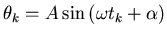
For example, consider the problem of estimating the amplitude and
phase of a signal at a known frequency,
, or within transcendental functions, such a
cosine).
Sometimes this linearity can be achieved by applying a transformation
to the original problem to arrive at a new problem which is linear.
For example, consider the problem of estimating the amplitude and
phase of a signal at a known frequency,
 |
|
|
(9) |
where  is known,
  and
and  are observed and where
 and
and  are to be estimated.
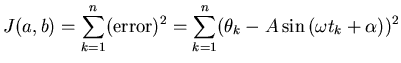
The simplest cost function would be
 |
|
|
(10) |
Our equations now give us,
These equations are hopelessly intertwined, the terms
cannot be pulled out into an equation for that is
separate from the in the same way that we achieved (7) and (8).
The direct solution of these
equations requires an approximation involving successive iterations
or some other method.
This problem fortunately has the nice property that it
can be transformed into another estimation problem which is linear.
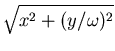
If we let,
then with a little trigonometry, we can write our unknowns and
as,
(as long as the amplitude and phase are constant, it does not matter
where in our data set we apply (13) and (14), so we drop the indexing
subscripts).
Now can we find an optimal estimate of  and
and  ? If so,
then we are all set. It turns out that we can.
The complicating factor here is that our
cost function must now account for the two components and ,
while we still are relying on the observations
? If so,
then we are all set. It turns out that we can.
The complicating factor here is that our
cost function must now account for the two components and ,
while we still are relying on the observations  .
.
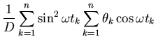
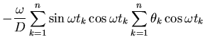
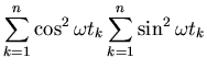
With lots of messy, tedious, but straightforward algebra we can
solve this problem to arrive at:
for
How does one come up with this kind of transformation for a new
problem ? There are a few fairly standard transformations that
you can use, for instance
can be converted to a straight line fit problem by taking the
logarithm of both sides. But mostly, finding a suitable
transformation is a matter of experiance, persistance and luck.
Next: Conclusion
Up: number10
Previous: Fitting data to a
Skip Carter
2008-08-20
![$\displaystyle -2 \sum_{k=1}^n \left[ \sin{ (\omega t_k + \alpha) }
( \theta_k - \sin{ (\omega t_k + \alpha) } ) \right] = 0$](img32.png)
![$\displaystyle -2 \sum_{k=1}^n A \left[ \cos{ (\omega t_k + \alpha) }
( \theta_k - A \sin{ (\omega t_k + \alpha) } ) \right] = 0$](img33.png)
![$\displaystyle \omega \left[ \sum_{k=1}^n \cos{\omega t_k} \sin{\omega t_k} \right]^2$](img52.png)