Fitting data to a Straight line

The simplest example of the application of least squares estimation is the fitting of data to a straight line. In this problem, our model of the system is the equation for a straight line,

$$y = a x + b$$ (1)

where $a$ and $b$ are the unknown adjustable parameters. If we let $z$ represent the measurements of what should be $y$, i.e.,

$$z = a x + b + \mbox{error}$$

then we can define our cost function as:

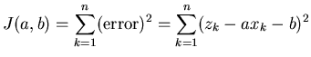$$J(a,b) = \sum_{k=1}^{n} (\mbox{error})^2 = \sum_{k=1}^{n} (z_k - a x_k - b)^2$$ (2)

To apply the least squares formalism to this, we need to figure out how to minimize $J$ with respect to $a$ and $b$. We do this by applying a little bit of calculus. The extreme values of a function (maximum and minimum) occur where the derivative is zero. The fact that it is straightforward to handle the derivative of a squared quantity is what makes using the square more attractive than the use of the absolute value. We have two parameters, so we need to calculate the derivatives with respect to both of them,

$$\frac{\partial J}{\partial a} = -2 \sum_{k=1}^n ( z_k - a x_k + b ) x_k = 0$$ (3)

$$\frac{\partial J}{\partial b} = -2 \sum_{k=1}^n ( z_k - a x_k + b ) = 0$$ (4)

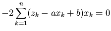
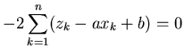
We need to expand these out and solve for $a$ and $b$ when both of these equations are simultaneously set to zero.

Now we have derived from (3),

$$0 = -2 \left[ \sum_{k=1}^n x_k z_k - (a + b )\sum_{k=1}^n x_k^2 \right]$$ (5)

and from (4),

$$0 = -2 \left[ \sum_{k=1}^n z_k - a \sum_{k=1}^n x_k - b n \right]$$ (6)

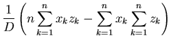
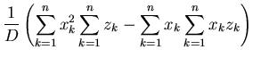
These can now be used to give equations for $a$ and $b$,

$$a = \frac{1}{D} \left( n \sum_{k=1}^n x_k z_k - \sum_{k=1}^n x_k \sum_{k=1}^n z_k \right)$$ (7)

$$b = \frac{1}{D} \left( \sum_{k=1}^n x_k^2 \sum_{k=1}^n z_k - \sum_{k=1}^n x_k \sum_{k=1}^n x_k z_k \right)$$ (8)

for,

$$D = n \sum_{k=1}^n x_k^2 - \left( \sum_{k=1}^n x_k \right)^2$$

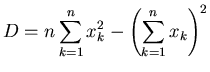
This is our optimal, least-squares, estimate of $a$ and $b$. Note we should verify that this solution is the minimum solution and not the maximum (remember that the first derivative is zero at both places). This verification requires taking the second derivatives and establishing that they are positive. This is pretty easy to show if one looks at (5) and (6). The second derivative of $J$ with respect to $a$ is the derivative with respect to $a$ of the right hand side of (5), which is $2 \sum x^2$. Since this is the sum of squared quantities it is positive so the second derivative is positive. Doing the same for $b$, we take the derivative with respect to $b$ of the right hand side of (6) and we get $2 n$, which again is positive.

Listing 1, shows an example of a general purpose least squares fit routine. It takes data pairs $(x,z)$ and returns the optimal estimates of $a$ and $b$. For the sample data file in listing 2, you should get a slope of 0.1781 and an intercept of 0.3687. With a sufficient amount of patience (or by putting Mathematica to work), we can work out equations like (7) and (8) for any polynomial form, not just a straight line.