Next: Conclusion, Part I
Up: number11
Previous: The controller equations
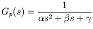
We will start with the Laplace transform of
the plant equation (5),
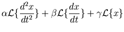
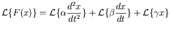
since its a little simpler to do. The first step is to use the
linearity property of Laplace transforms, which is given as the third
rule in Table 2. This property allows us to do the transform of (5)
by doing the transform of each term separately,
 |
|
|
(6) |
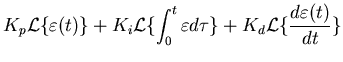
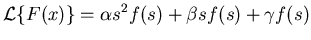
and further the linearity property allows us to move the constants
outside of the transform operation,
Now representing
 as
as  , we get,
 |
|
|
(8) |
The transfer function is the ratio of the output response to
the input forcing
 , which we get by rearranging
the above equation to get,
, which we get by rearranging
the above equation to get,
 |
|
|
(9) |
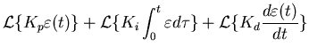
Now that we see how we go about doing this, its a straightforward
matter to do the same for the PID controller,
(we needed the derivative rule, number 4, and the integral
rule, number 7, from Table 2 as well as the linearity rule).
Now we have to be careful here, the transfer function is the
ratio of the output to the input. For the PID controller the
error signal,  , is the input, the output
is the quantity
, is the input, the output
is the quantity  .
.
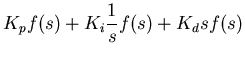
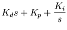
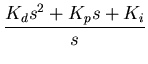
So the transfer function is for the PID controller is,
Now we need to couple the controller and the plant. We will
connect the output of the controller into the plant by taking
the controller output, multiplying it by a plant gain factor
 , and using that as the plant input. This is represented
mathematically by multiplying the controller response by the
plant gain and the plant response,
, and using that as the plant input. This is represented
mathematically by multiplying the controller response by the
plant gain and the plant response,
We will connect
the plant output into the controller at the negative side
of the summing node (to get an error signal) after multiplying
it by a feedback gain factor  .
The plant and feedback gains do not really change anything, they
just give us more opportunities to adjust things. The real change
is the fact that the input to the controller is now reinterpreted
as the output of the summing point (before is was just ``the input'',
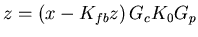
now we care how it relates to the rest of the system). So now
part of the system input is the system output,
.
The plant and feedback gains do not really change anything, they
just give us more opportunities to adjust things. The real change
is the fact that the input to the controller is now reinterpreted
as the output of the summing point (before is was just ``the input'',
now we care how it relates to the rest of the system). So now
part of the system input is the system output,
We get the full equation by going step at a time through the
diagram (figure 1).
At the output of the summing node we have,
then after the controller we get,
and so after the plant we have,
 |
|
|
(12) |
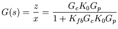
The response function is the ratio of the output to the input
 which we can determine by reorganizing the above equation
to get,
which we can determine by reorganizing the above equation
to get,
 |
|
|
(13) |
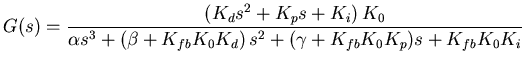
now we expand this using (9) for  and (11) for
  and
simplify,
and
simplify,
 |
|
|
(14) |
This is the response function of our PID controller with the plant
defined by equation (5). Notice that we managed to go from a
description of how the controller is interconnected (basically Figure
1) all the way to its input response function with nothing more than
polynomial manipulations. If we had not used Laplace tranforms,
getting the response function by the
direct manipulations of the integro-differential equation would have
been much harder to do.
It is important to recognize that the details of what we have done
are dramatically dependent upon the forms of equations (4) and (5).
However the method that we used will apply as long as the two
equations (and how they are coupled) are linear.
Now that we know how the adaptive controller will respond, how do
we adapt it ? First we need to understand what it means for the
controller to be optimally adapted.
To do this, we need to consider when the denominator
of equation (14) is zero.
 |
|
|
(15) |
This equation is called the characteristic equation for the
system. For the moment we will combine the coefficients,
 |
|
|
(16) |
The locations of the solutions to (16) in the complex plane can be
used to predict the behaviour of the controller. For a given
set of coefficients, there will be three solutions called the roots.
If the roots are in the negative half of the plane, then the
controller will be stable.
If the roots are real but unequal, then the system is overdamped
(that is, it will never quite recover from a suddenly imposed step
input). If the roots are imaginary, then the system is underdamped
(which will ``ring'' when it gets a step input). The optimal
response to an imposed step is the critically damped case, this
will happen if the roots are real and equal.
So our goal is to adjust the gains (the various  values) so that
the characteristic equation always has real, equal, negative roots.
It turns out that we can achieve all these constraints provided
that in equation (16),
values) so that
the characteristic equation always has real, equal, negative roots.
It turns out that we can achieve all these constraints provided
that in equation (16),  and
and  have opposite signs and that
Clearly, we cannot optimally adaptively control an arbitrary plant.
If  and
and  don't have opposite signs then the controller
won't even be stable. Also note that there are not enough equations
to give us independently all five gains. The feedback and plant
gains and are either going to have to be defined to
have fixed (known) values or they will need to be absorbed into
the other gains.
don't have opposite signs then the controller
won't even be stable. Also note that there are not enough equations
to give us independently all five gains. The feedback and plant
gains and are either going to have to be defined to
have fixed (known) values or they will need to be absorbed into
the other gains.
Next: Conclusion, Part I
Up: number11
Previous: The controller equations
Skip Carter
2008-08-20