The importance of being linear

While there is a good deal of mathematics behind adaptive controllers, its not particularly hard mathematics. The reason for this is that traditionally most controllers are linear. We can take advantage of this linearity to make the equations relatively easy to manipulate. Lets first consider what is means for a system to be linear. Essentially, linearity means that the system obeys a superposition principle. Suppose that $f(.)$ represents our system and further that $A$ and $B$ are two valid but otherwise arbitrary solutions to $f$. Then if it is true that,

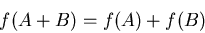$$f(A + B) = f(A) + f(B)$$ (1)

then the system is said to be linear. Many familiar systems have this property. It is equation (1) that allows us to decompose a periodic signal into frequency bands and calculate a power spectrum. Potential fields (electric, magnetic and gravitational) are also linear. The main reason why linear systems are so familiar, is not because they are so ubiquitous (in fact, one author has pointed out that dividing nature into linear and nonlinear systems is like having ``nonelephant'' biology as a special subfield, and missing the fact that most systems are not linear), but because equation (1) makes linear systems solvable. Many nonlinear systems are handled by making them approximately linear, e.g.:

$$f( A + B ) = f(A) + f(B) + \mbox{ a little bit extra }$$ (2)

The work then primarily concentrates on how small that little bit actually is and under what circumstances is stays small. For many nonlinear systems (2) is a practical approach that gives useful answers. Systems that can be analyzed this way generally get described with phrases like ``small amplitude''; a dead giveaway that something like (2) was used. A simple example of this is the ordinary pendulum. A pendulum is actually a nonlinear system, but for small amplitude excursions (say 10 degrees), the nonlinear effects are extremely small and can be ignored for typical applications. Some nonlinear systems cannot be broken down to something like (2) without completely missing the real solutions. Any system that has chaotic behavior is like this, the chaos comes from the nonlinearity; there are no chaotic systems that are linear.

Many methods have been invented for dealing with linear systems, one that we will find useful here is the Laplace transform. For the system $F(t)$ the Laplace transform ${\mathcal{L}}\{F(t)\}$ is defined by,

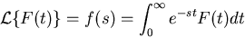$${\mathcal{L}}\{F(t)\} = f(s) = \int_0^{\infty} e^{-st} F(t) dt$$ (3)

(strictly speaking this applies only for $t > 0$). There are two properties that make the Laplace transform particularly suited to our problem:

• Like the Fourier transform, it converts a linear differential equation into a polynomial. (you might not have realized this, but we can transform - Fourier or Laplace - an equation, not just a stream of data).
• Unlike the Fourier transform, it treats transients efficiently. The Laplace transform is, in fact, the impulse response function for a system.

Its a bit tedious to do the integrations required to do either a forward or inverse transform by hand, so the Laplace transform is often done with the help of symbolic integration software or the use of tables in a handbook. Table 1 gives the Laplace tranform for several useful mathematical functions. Combining this with some general transformation properties given in Table 2, gives us the ability to determine the Laplace tranform of a large number of useful functions without the need to explicitly solve (3). The forward Laplace transform is not too difficult to do numerically, but calculating the inverse transform numerically leads to problems with the numerical stability of the calculation; this is not a problem with software that is capable of doing the inverse tranform symbolically.

We will use the Laplace tranform to work out how the controller will respond to its inputs. We need to do be able to do this because there is no unique way to set up an adaptive controller - a motor speed controller that uses a shaft angle encoder will be quite different from one that uses a tachometer.