


Next: The LMS adaptive filter
Up: number9
Previous: General principles
The simplest error signal that we can generate is
just the difference between what we are getting out of the filter,
 ,
and what we expect to see,
,
and what we expect to see,  ,
,
 |
(1) |
For many problems an overshoot is just as bad as an undershoot,
so we can use the mean square error as a cost function.
There are lots of other cost functions that we could use, but this
one is particularly convienient mathematically.
The earliest adaptive filter derived from this error and cost
function is the Wiener filter. Unfortunately, it is in
FIR form and has coefficients that extend infinitely back
in time. Except for certain periodic systems, this filter is
not very practical. The filter can be rederived in IIR
form, this is known as the Kalman filter. The discrete
time, linear, form of this equation looks like,
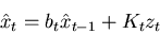 |
(2) |
 , is a model of how the system goes from one time interval
to the next. It is our best understanding of how the ideal system
goes from a value at time
, is a model of how the system goes from one time interval
to the next. It is our best understanding of how the ideal system
goes from a value at time  to a value at time
  .
.
 is the Kalman gain, it is not controlled by the
measurements directly, but instead is determined by how good you
think the model
is the Kalman gain, it is not controlled by the
measurements directly, but instead is determined by how good you
think the model  is as compared to the quality of the observations.
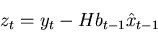
 is called the innovation, it is an estimate of what
you think the error will be at time , given a measurement
at time ,
is called the innovation, it is an estimate of what
you think the error will be at time , given a measurement
at time ,  , and a prediction of
  at time based upon the
best estimate of at extrapolated to time by applying
our model funtion, . The simplest example of how to calculate
the innovation is,
at time based upon the
best estimate of at extrapolated to time by applying
our model funtion, . The simplest example of how to calculate
the innovation is,
 |
(3) |
where  is a function that may be necessary to convert the
components of to the components of
is a function that may be necessary to convert the
components of to the components of  (An example is the
meteorological case of
estimating the humidity (the ) based upon wet-bulb and dry-bulb
temperature measurements (the ). The function would have one
component that converts humidity to wet-bulb temperature, and one
for the conversion to dry-bulb).
In an application, the innovation is a known function, like above,
and the function is known. What is not known is the
gain,
(An example is the
meteorological case of
estimating the humidity (the ) based upon wet-bulb and dry-bulb
temperature measurements (the ). The function would have one
component that converts humidity to wet-bulb temperature, and one
for the conversion to dry-bulb).
In an application, the innovation is a known function, like above,
and the function is known. What is not known is the
gain,  ; this must be calculated in parallel with the model
estimation. The time varying gain is where the adaptative nature
of the Kalman filter expresses itself.
; this must be calculated in parallel with the model
estimation. The time varying gain is where the adaptative nature
of the Kalman filter expresses itself.
In order to determine the equation that gives us the gain function,
we have to spend some time with optimal estimation theory. I will
not spend the time on this here, but just show the the result.
In the scalar case, the gain function is:
![\begin{displaymath}
K_t = \frac{ H \left[ b^2 p_{t-1} + \sigma^2_g \right] }
{ \sigma^2_\nu + H^2 \sigma^2_g + H^2 b^2 p_{t-1} }
\end{displaymath}](img17.png) |
(4) |
Two of the new quantities,  and
and  , are
the noise or error variances for the model, , and the measurements
respectively. The first is a statement about how good you believe
the model of the system is. The second quantifies how good you think
your measurements are. Both of these quantities are presumed to be
known. The third quantity,
, are
the noise or error variances for the model, , and the measurements
respectively. The first is a statement about how good you believe
the model of the system is. The second quantifies how good you think
your measurements are. Both of these quantities are presumed to be
known. The third quantity,  , is the error covariance of
the filter, it gives effectively the error bars of the current
model output. This can be calculated given the gain,
, is the error covariance of
the filter, it gives effectively the error bars of the current
model output. This can be calculated given the gain,
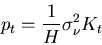 |
(5) |
To use the filter, each time a new observation () becomes
available we calculate (3) and (4), and then use that information
in (2) and (5).
The Kalman filter is frequently applied to systems where and
are multi-channel or vector systems. In this case
the equations (2) through (5) are rewritten as matrix equations.
Next: The LMS adaptive filter
Up: number9
Previous: General principles
Skip Carter
2008-08-20