Next: Conclusion
Up: number8
Previous: The Z Transform
Having established the convolution theorem is very
important since digital filters can be described in terms of
convolutions. The Z transform version allows us to work with these
filters by merely manipulating polynomials. In order to see that
this is so, I have to reveal one neat fact about the Z transform.
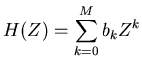
The Z transform that we have describe above can be written as,
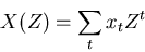 |
(9) |
If this is evaluated on the unit circle in the complex plane, that
is we let
 , then we get
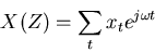 |
(10) |
which is the definition of the (discrete) Fourier transform!
In other words the Fourier transform is just the Z transform
evaluated on the unit circle.
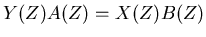
So one way to interpret (7), is that we can make  be a series
that has a spectrum that is the spectrum of
be a series
that has a spectrum that is the spectrum of  modified by the
spectrum of
modified by the
spectrum of  . So for example if we design to have a zero
at 60 Hz, then will be the signal with 60 Hz removed, i.e.
we have a notch filter.
. So for example if we design to have a zero
at 60 Hz, then will be the signal with 60 Hz removed, i.e.
we have a notch filter.
In general we can write a digital filter in the form,
 |
|
|
(11) |
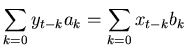
or written out in the time domain,
 |
|
|
(12) |
If represents the measurement data and  and are the
(somehow) known filter coefficients then the above equation can
be reorganized in a way that is more obviously useful,
and are the
(somehow) known filter coefficients then the above equation can
be reorganized in a way that is more obviously useful,
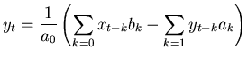 |
|
|
(13) |
This equation is a general formulation of a digital filter. If the
coefficients beyond  are nonzero, it is called an
Infinite Impluse Response (IIR) filter because an input series
consisting of all zeros except at one point will result in an
output series that will always contain some amount of the
original input (for real computers with finite CELL sizes
the output will actually eventually decay away because of truncation
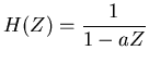
effects). An example IIR filter is what is known as the
leaky integrator,
are nonzero, it is called an
Infinite Impluse Response (IIR) filter because an input series
consisting of all zeros except at one point will result in an
output series that will always contain some amount of the
original input (for real computers with finite CELL sizes
the output will actually eventually decay away because of truncation
effects). An example IIR filter is what is known as the
leaky integrator,
For the special
case where the coefficients beyond are all zero, the
filter is called a Finite Impluse Response (FIR) filter because an
impulsive input will cause an output that will eventually settle down
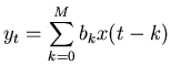
to a steady state. A simple example is the running average,
Everything that one can know about a digital filter is contained in
the ratio of elements the of  and
and  ,
,
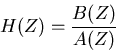 |
(14) |
which is known as the filter characteristic.
Foremost is the power transfer function which describes what
fraction of energy at a given frequency in the input appears in
the output,
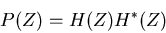 |
(15) |
where  is the complex conjugate (the sign of the imaginary
part is inverted) of
is the complex conjugate (the sign of the imaginary
part is inverted) of  .
.
Recall that in an earlier column, I pointed out the the power transfer
function is only part of the story. One should also consider what
the filter does to the phase of the input. In general a filters
effect on the phase is frequency dependent and so there is a
phase transfer function,
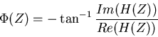 |
(16) |
The filter can also have an effect on packets of waves. These
packets are what you get, for example, when you modulate a one
frequency by another. The frequency of the modulation envelope
itself becomes a filterable component with its own transfer
function, the group transfer function,
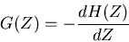 |
(17) |
All of these transfer functions are conventionally computed on the
unit complex circle.
The characteristic function for the leaky integrator is,
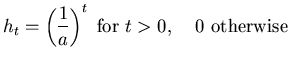
Converting this to the time domain gives the impulse response of
the filter,
For the running average filter, the function is,
and its impulse response is
Certain forms for the polynomials and have proven to be
useful and are widely used. For example the bandpass Butterworth
filter has the coefficients in the form,
The Butterworth filter chooses to optimize the flatness of the
bandpass region of  and in doing so gives up simple forms
for
and in doing so gives up simple forms
for  and
and  .
.
Chebyshev filters are designed to give the sharpest possible
transition between the bandpass and bandstop regions. The filter
gets its name because the filter characteristic contains a special
polynomial known as a Chebyshev polynomial,  .
.
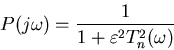 |
(19) |
This filter gains in the sharp transition by compromising on the
flatness of the bandpass region.
Elliptical or Cauer filters get even sharper transitions than
Chebyshev filters, but achieve this at the expense of ripples in
both the pass and stop bands. The filter characteristic
looks like the Chebyshev filter, except the Chebyshev polynomial
gets replaced by a Chebyshev rational function.
Bessel filters are designed with the goal of achieving the
flattest possible group delay. This results in a filter
has no ringing when it receives a step or impulse input.
The characteristic function for the  th order Bessel filter is
given by,
th order Bessel filter is
given by,
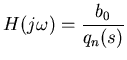 |
|
|
(20) |
where,
Next: Conclusion
Up: number8
Previous: The Z Transform
Skip Carter
2008-08-20