Sampling a time dependent signal

The problems involved in handling a more general time dependent signal, say a digitized acoustic signal, are considerably trickier. A primary problem is how to make the measurements without high frequency aliasing distorting the result. The problem is that if 2 $\times$ n is the sample rate, there is no way to distinguish a signal of frequency n from a signal of 2n (or any other integer multiple of n) because in both cases one sees a full cycle in two samples. In the 2n case there was a whole cycle in between our samples that we missed. This means that if we are sampling at 2 $\times$ n, there is a whole range of frequencies from n upward that can contaminate our measurements. This spurious folding of high frequencies down to a lower one is called aliasing. One can reduce this problem somewhat by sampling at a high rate, the idea being that it will increase the frequency at which aliasing begins to occur and one hopes that there is less of the higher frequency around to bother us. The problem is that it might not be the case that there is less at the higher frequency, and even worse this solution uses more CPU resources. A better solution is to prevent the high frequencies from getting into your samples in the first place. This is done by placing an anti-aliasing filter in the analog circuit before the A/D converter. An anti-aliasing filter is just a low pass filter designed to reject frequencies above n.

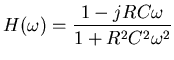
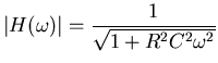
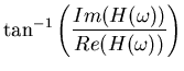
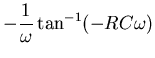
Anti-aliasing filters are frequently implemented as simple R-C filters like in Figure 1. This filter is not that great as filters go, the rate of attenuation of the higher frequencies is rather slow. The fraction of the signal passed through the filter as a function of frequency is called the magnitude response. The magnitude response curve is an important measure of the quality and suitability of a filter. Unfortunately, it is often used as the only measure. There is another measure that can be just as important to consider, the frequency dependent effect the filter has upon the phase of the signal. This is the phase response. The phase response information is most useful in two forms, the phase delay and the group delay. The phase delay is just a dimensional form of the phase response, it gives the amount of time a signal of a given frequency is delayed by the filter. The group delay describes something slightly different. Suppose our signal is like an FM radio signal, that is being modulated in frequency around a basic frequency. The modulation can be thought of as another signal (the envelope) riding on top of the basic frequency (the carrier). The phase delay of the envelope is not generally the same as the phase delay of the carrier. The group delay gives the delay time of the envelope. So to properly judge the suitability of a given filter we really need to check all three functions: the magnitude response, the phase delay and the group delay. As you might expect, all filters give up performance in one of the three functions in order to gain in another. The best compromise depends upon your application.

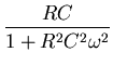
All of these filter characteristics can be derived from the filters transfer function. This is a complex function (that is, it contains complex numbers in it) and takes a bit of mathematics to be able to derive for an aribitrary filter. I will only give you the results here for the low-pass RC filter. If you are interested in learning more about this, Horowitz and Hill contains a readable introduction to the topic. The low-pass RC filter has a the transfer function,

$$H(\omega) = \frac{ 1 - j R C \omega}{1 + R^2 C^2 \omega^2}$$

here I have used the engineers notation for the $\sqrt{-1}$, $j$, and not the scientists notation, $i$. The term $\omega$ is the frequency in radians, to get Hertz divide $\omega$ by $2 \pi$. With this equation, we can get the magnitude response,

$$\vert H(\omega) \vert = \frac{1}{\sqrt{1 + R^2 C^2 \omega^2}}$$

the phase response is,

$$\theta( \omega ) = \tan^{-1} \left( \frac{ Im( H( \omega ) ) } { Re( H( \omega ) ) } \right)$$

$$= \tan^{-1}( R C \omega )$$

So the phase delay is,

$$\tau_p (\omega) = - \frac{ \theta(\omega) }{ \omega }$$

$$= - \frac{1}{\omega} \tan^{-1} ( - R C \omega )$$

and the group delay is,

$$\tau_g (\omega) = - \frac{ d \theta(\omega)}{d \omega }$$

$$= \frac{ R C }{ 1 + R^2 C^2 \omega^2}$$

With the anti-aliasing filter in place, we still need to decide upon the proper sampling rate. You might recall reading elsewhere about something called the Nyquist sampling theorem. This theorem is what we want, it tells us that the sample rate must be at least twice the bandwidth of the signal in order to avoid aliasing. Notice that I said bandwidth, which is the range from the lowest to the highest frequency (in the simplest case, where there are no gaps) in the signal. The Nyquist theorem is widely misquoted as stating that we must sample at twice the highest frequency of the signal. The bandwidth and the highest frequency are not the same thing unless we are dealing with a base band signal (one that has content from a frequency of zero all the way up to the highest frequency). The distinction can be quite important. Consider the following real-life example. In the RAFOS subsurface ocean drifter, that I helped develop, we navigate the float by listening to a tone emitted by a pre-placed acoustic beacon mooring. These beacons output a long tone that sweeps in frequency from 258.5 to 261.5 Hertz. The bandwidth of this tone is the range of the sweep, 3 Hertz. So the Nyquist theorem states that we need a sampling rate of at least 6 Hertz, not at twice the highest frequency of 261.5 Hz (523 Hz). As a result, the RAFOS float can comfortably oversample the signal at 10Hz using a lowly 6805 microprocessor. Erroneously sampling at 523 Hz would have required a faster processor, which would have required more electrical power which, in turn, would make the instrument an impractical device (the drifter runs on batteries and has mission times measured in months, 48 being our current record).

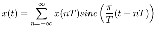
If we are uniformly sampling a signal at the proper rate, and there is no aliased signal contaminating our measurement, then we can recover the value of the signal at any time. To do this we need to do a convolution of our samples with the sinc function (this is the uniform sampling theorem),

$$x(t) = \sum_{n = -\infty}^{\infty} x( nT ) sinc\left( \frac{\pi}{T} (t - nT) \right)$$

where $t$ is the time we want to reconstruct the signal at, $T$ is the interval between samples, and $n$ is the sample index. (I am not going to explain the mathematics behind this here. It could provide material for several future columns to explain it. If you want to research this on your own the book by Bracewell is highly recommended). In order to make practical use of this equation we will take the index $n$ over the number of data samples, instead of infinity.

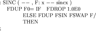
A Forth implementation of the sinc function is,

By the way, if you look up equations like these in the literature I can guarantee you will have a horrible time reconciling factors of $\pi$, 2, and -1 ( this is generally known as the $\pi$ throwing contest. Where did the $\pi$ go ?). In the mathematics literature these factors tend to be missing from the equations altogether. In the engineering literature they are in different places in different books. The reason is that such factors are immaterial as far as the mathematical theory of all this is concerned, they are just normalization and dimensionalization factors. In the engineering context, there is no one way to do normalization and dimensionalization they just need to be done self consistently; so one books version can differ from anothers.

Now that we are armed with the uniform sampling theorem, we can do a little experiment to demonstrate what I said about sampling a bandlimited signal. Listing 2, gensig.fth is a program that will generate a test signal that starts at one frequency and slides up to another (a chirp). I have set things up so that the simulated signal sweeps from 10 Hz to 12 Hz in 4.5 seconds. When the constant SAMPLING? is FALSE then the output is at the equivalent of 128 samples per second.

A subsample of the output of this program is what we will be using as data, a plot is shown in Figure 2. This signal has a bandwidth of 2 Hz, so the Nyquist sampling rate is 4 Hz. We will oversample and sample at 6.4 Hz. Now we can't just take every 20th sample from the data in Figure 2 to use as our measurement data; such a signal would contain a serious amount of aliasing in it. To make the signal usable, we will mix it with an 11 Hz signal and then apply a low-pass filter with a 5 Hz cut-off to the result.

Why do we do that ? From elementary trigonometry,

$$2 \times sin(x) \times cos(y) = sin(x-y) + sin(x+y)$$

which means that if we take a signal of one frequency, $x$, and multiply it by another signal of frequency, $y$, then we end up with one signal with frequency $x-y$, and another at $x+y$. So if $x$ is our original signal which sweeps from 10 to 12 Hz, and $y$ is a fixed signal at 11 Hz, then we end up with a signal centered at 0 Hz and another at 22Hz. The one at 0 Hz is the one we want to keep, the other at 22Hz we will filter out. This technique for shifting the center frequency of a signal is the heart of what is known as a heterodyne mixer. The special case where we shift to a center frequency of zero is known as a homodyne mixer. After mixing and filtering the original signal, we can then safely subsample it. The anti-aliasing filter being used here is a first-order low-pass Butterworth filter. There are better choices for the filter (such as a Bessel filter), but I am using it here because it is simple and it illustrates a point which we will get to later. All of these operations are in the code gensig.fth when the constant SAMPLING? is set to TRUE.

The output for the sampling case are the simulated measurements that we want to use the uniform sampling theorem upon. The code in regen.fth (listing 3) reads the data and applies the theorem to it. Comparing the output of regen with its input we see a smoother result as one might expect. In order to see what we theoretically expect, go back and run gensig with SAMPLING? set to FALSE and the minimum and maximum frequencies set to -1.0 and 1.0 respectively. Running gensig this way generates the reference signal without the 11Hz carrier.

Comparing the carrier free signal with the reconstructed signal (figure 3), we see that we generally do pretty well. There are two problems that we can see with our reconstruction:

• The end points aren't that well matched. In this example the starting end looks very good, but that is an artifact of the fact that the signal starts off at zero. The end point problem is due to the fact that the theorem we are using assumes that there is data on both sides of our estimation point (and in fact an infinite amount of it), but as we near the edges the calculation gets most of its information from only one side of the point. More data helps here, but the end points are always going to be a problem.
• The reconstruction is slightly phase shifted late. If you look carefully you'll notice that the phase shift is in the measurement data and that the reconstruction has the same shift. This is because the phase shift is caused by the anti-aliasing filter. The group delay of the Butterworth filter that is being used here is frequency dependent. It starts at zero and monotonically increases until about 10 Hz; at 2 Hz it is about 0.05 seconds. This is a good example of where the group delay characteristics are more important than how sharp the high frequency cutoff is.