The controller equations

Recall from ``Closing the loop'' (FD XVIII No. 5) the equation for a proportional-integral-derivative (PID) controller is:

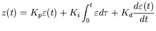$$z(t) = K_p \varepsilon(t) + K_i \int_0^t \varepsilon d\tau + K_d \frac{d \varepsilon(t)} {d t}$$ (4)

where $K_p$ is the proportional gain, $K_i$ is the integral gain and $K_d$ is the differential gain.

The quantity $\varepsilon$ is an error signal that is the difference between the commanded input, $x$ and the output of the controlled system $y$. In our earlier investigations we were not much concerned with the internals of the controlled system (often called the plant), all we needed was the output signal. Figure 1 shows a generic schematic of our controller and plant.

For an adaptive system, we need to have an additional equation that describes how the plant behaves so that we can properly adjust the parameters of the controller. So now we have two equations to consider, the controller and the plant. The design of the adaptiveness depends upon the form of both equations. For our example plant, we will use the second order differential equation:

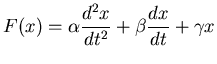$$F(x) = \alpha \frac{d^2 x}{d t^2} + \beta \frac{d x}{d t} + \gamma x$$ (5)

this is a pretty generic model, as a example this can be thought of as a damped mass-spring system where $\alpha$ is the mass, $\beta$ is the friction and $\gamma$ is the spring constant. $F(x)$ would represent the imposed external forces on the system (the input), and the solution to the equation would give the plants response to it.